pacman::p_load(tidyverse, rpart, rpart.plot, sparkline, visNetwork,
caret, ranger, patchwork)Decision Tree
Load Packages and Data
As there are too many levels within the variable Country (and Code), this variable will be removed from the regression data set.
Similarly, ID cannot be used as a predictor, hence, will be removed.
df <- read_csv("data/touristdata_clean.csv")

df_analysis <- df %>%
  select(!ID) %>%
  select(!code) %>%
  select(!country)
Regression Tree
Basic Regression Tree model
anova.model <- function(min_split, complexity_parameter, max_depth) {
  rpart(total_cost ~ .,
        data = df_analysis,
        method = "anova",
        control = rpart.control(minsplit = min_split,
                                cp = complexity_parameter,
                                maxdepth = max_depth))
  }

fit_tree <- anova.model(5, 0.001, 10)
Visualising the Regression Tree
visTree(fit_tree, edgesFontSize = 14, nodesFontSize = 16, width = "100%")Tuning of hyperparameters
printcp(fit_tree)
Regression tree:
rpart(formula = total_cost ~ ., data = df_analysis, method = "anova",
    control = rpart.control(minsplit = min_split, cp = complexity_parameter,
        maxdepth = max_depth))

Variables actually used in tree construction:
 [1] age_group                 info_source
 [3] main_activity             most_impressing
 [5] night_mainland            night_zanzibar
 [7] package_accomodation      package_food
 [9] package_guided_tour       package_insurance
[11] package_transport_int     payment_mode
[13] prop_night_spent_mainland purpose
[15] region                    total_female
[17] total_male                total_night_spent
[19] total_tourist             tour_arrangement
[21] travel_with

Root node error: 7.0099e+17/4762 = 1.472e+14

n= 4762

          CP nsplit rel error  xerror     xstd
1  0.2221822      0   1.00000 1.00035 0.052747
2  0.0653800      1   0.77782 0.77839 0.043901
3  0.0312447      2   0.71244 0.71425 0.040452
4  0.0098871      4   0.64995 0.65256 0.037716
5  0.0089989      6   0.63017 0.67161 0.039356
6  0.0089654      7   0.62118 0.66769 0.039297
7  0.0066781      8   0.61221 0.66470 0.039580
8  0.0056746      9   0.60553 0.67466 0.039909
9  0.0055600     10   0.59986 0.67718 0.040160
10 0.0053787     11   0.59430 0.67538 0.040073
11 0.0053253     12   0.58892 0.67416 0.040067
12 0.0051713     13   0.58359 0.67792 0.040474
13 0.0048403     14   0.57842 0.69170 0.042433
14 0.0046831     15   0.57358 0.68878 0.042367
15 0.0045494     16   0.56890 0.68910 0.042361
16 0.0045415     17   0.56435 0.68977 0.042426
17 0.0038489     19   0.55527 0.69473 0.042914
18 0.0037768     20   0.55142 0.69775 0.042964
19 0.0036528     21   0.54764 0.70032 0.043070
20 0.0036431     24   0.53668 0.70148 0.043066
21 0.0035646     28   0.52211 0.70398 0.043207
22 0.0032389     29   0.51855 0.71428 0.043857
23 0.0028148     30   0.51531 0.72328 0.043775
24 0.0027982     31   0.51249 0.72319 0.043778
25 0.0027464     35   0.50130 0.72493 0.043572
26 0.0026194     37   0.49581 0.72545 0.043583
27 0.0025449     38   0.49319 0.72538 0.043533
28 0.0021832     39   0.49064 0.72313 0.043377
29 0.0021695     40   0.48846 0.72965 0.043468
30 0.0020550     41   0.48629 0.73039 0.043476
31 0.0019419     42   0.48423 0.73965 0.043711
32 0.0019108     43   0.48229 0.73918 0.043661
33 0.0018682     44   0.48038 0.73532 0.043332
34 0.0017684     45   0.47851 0.74036 0.043480
35 0.0016929     47   0.47498 0.74145 0.043512
36 0.0016091     51   0.46820 0.74680 0.044044
37 0.0015919     54   0.46338 0.74660 0.044052
38 0.0015800     55   0.46179 0.74778 0.044085
39 0.0015561     56   0.46021 0.75098 0.044145
40 0.0014456     58   0.45709 0.75257 0.044020
41 0.0014314     63   0.44986 0.75931 0.044191
42 0.0013349     64   0.44843 0.76174 0.044228
43 0.0013221     66   0.44576 0.75808 0.044075
44 0.0012398     67   0.44444 0.75845 0.044210
45 0.0011227     69   0.44196 0.76544 0.044336
46 0.0010561     70   0.44084 0.76868 0.044382
47 0.0010518     74   0.43661 0.76927 0.044405
48 0.0010445     75   0.43556 0.76857 0.044400
49 0.0010335     76   0.43452 0.77047 0.044420
50 0.0010176     77   0.43348 0.76988 0.044414
51 0.0010152     78   0.43247 0.76970 0.044413
52 0.0010000     79   0.43145 0.76864 0.044381
bestcp <- fit_tree$cptable[which.min(fit_tree$cptable[,"xerror"]),"CP"]
pruned_tree <- prune(fit_tree, cp = bestcp)
visTree(pruned_tree, edgesFontSize = 14, nodesFontSize = 16, width = "100%")Random Forest
Splitting of data set into train vs. test data
set.seed(1234)

trainIndex <- createDataPartition(df_analysis$total_cost, p = 0.8,
                                  list = FALSE,
                                  times = 1)

df_train <- df_analysis[trainIndex,]
df_test <- df_analysis[-trainIndex,]
Hyperparameter Tuning and Training of Model
##setting option for user to decide if they want to do parameter tuning
##default is simple bootstrap resampling
trctrl <- trainControl(method = "none")

##alternative is (repeated) k-fold cross-validation - user input decision on the value of k and the number of repeats
cvControl <- trainControl(##default of 10, range: 3-50
                           method = "cv",
                           number = 10)

repeatcvControl <- trainControl(##default of 10, range: 3-50
                           method = "repeatedcv",
                           number = 10,
                           ##default of 3, range: 3-10
                           repeats = 10)

##building of model
rf_model <- train(total_cost ~ .,
                  data = df_train,
                  method = "ranger",
                  trControl = repeatcvControl,
            #trControl (refer to above objects created)
                  num.trees = 50, #can consider range of 5 to 200 trees
                  importance = "impurity",
            #variable importance computation: "impurity", "permutation"
                  tuneGrid = data.frame(mtry = sqrt(ncol(df_train)),
                                        min.node.size = 5,
                                        splitrule = "variance")
            #splitrule: "variance" (default), "extratrees", "maxstat", "beta"
            #min.node.size: default of 5 for regression trees
            #mtry: default is square root of number of variables
                  )
Visualising of predicted vs. observed responses
##Fit test data into the model that has been built
df_test$fit_forest <- predict(rf_model, df_test)

##Scatterplot of predicted vs. observed and Residuals scatterplot
rf_scatter <- ggplot() +
  geom_point(aes(x = df_test$total_cost, y = df_test$fit_forest)) +
  labs(x = "Actual Total Cost", y = "Predicted Total Cost",
       title = paste0("R-squared: ", round(rf_model$finalModel$r.squared, digits=2))) +
  theme(axis.text = element_text(size = 5),
        axis.title = element_text(size = 8),
        title = element_text(size = 8))

rf_residuals <- ggplot() +
  geom_point(aes(x = df_test$total_cost,
                 y = (df_test$fit_forest-df_test$total_cost)),
             col="blue3") +
  labs(y ="Residuals (Predicted-Actual)", x = "Actual Total Cost") +
  geom_hline(yintercept = 0, col="red4", linetype = "dashed", linewidth = 0.5) +
  theme(axis.text = element_text(size = 5),
        axis.title = element_text(size = 8))

p <- rf_scatter + rf_residuals +
  plot_annotation(title = "Scatterplot of predicted vs. actual total cost",
                  theme = theme(plot.title = element_text(size = 18)))

p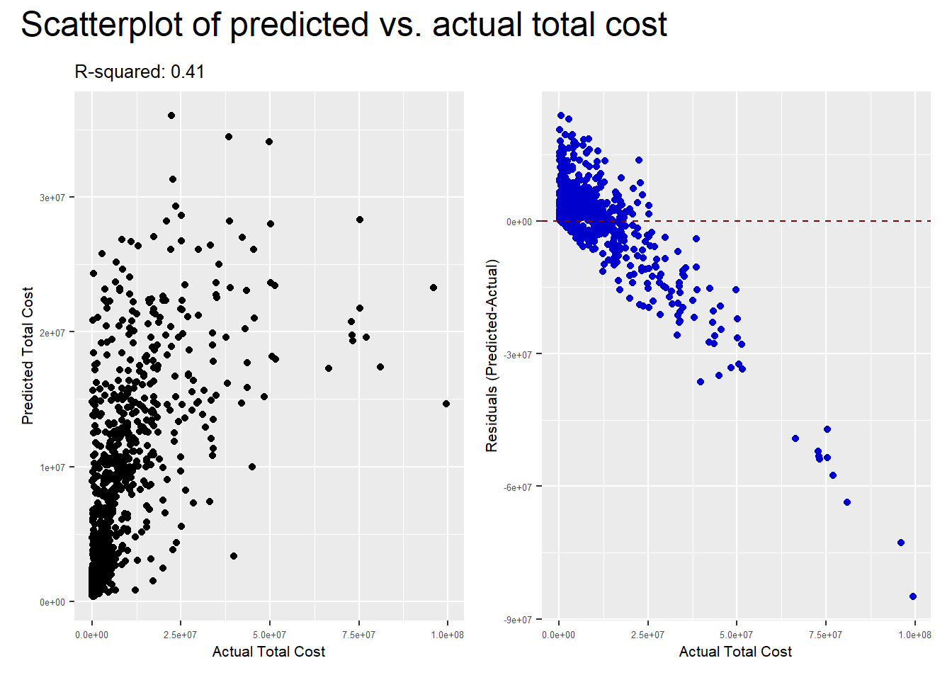
Visualising variable importance (top 20)
varImp(rf_model)ranger variable importance
only 20 most important variables shown (out of 57)
Overall
total_tourist 100.00
total_night_spent 76.30
package_transport_tz 70.21
package_transport_int 69.69
tour_arrangementPackage Tour 64.64
total_female 57.60
night_mainland 54.91
total_male 52.75
night_zanzibar 41.79
package_accomodation 40.91
package_food 39.31
prop_night_spent_mainland 37.94
package_guided_tour 35.47
travel_withSpouse and Children 30.47
purposeLeisure and Holidays 28.00
regionEurope 26.14
age_group65+ 24.34
package_sightseeing 24.17
regionAmericas 23.69
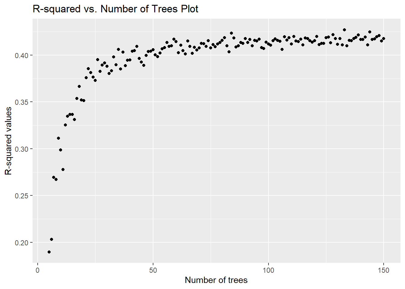
info_sourceTravel, agent, tour operator 22.72Visualising of R-squred value vs. the number of trees
The original intention was to take in an input range for the number of trees and build a chart that would show a summary of how the R-squared value changes accordingly for the model trained above.
However, after an attempt to build the chart on the Shiny app, we realised that the app may not have sufficient memory space to handle the for loop required to build this chart. As such, this chart is dropped from the final Shiny app.
tree_range <- 5:150

rsquared_trees <- c()

for (i in tree_range){
  rf_model <- train(total_cost ~ .,
                  data = df_train,
                  method = "ranger",
                  trControl = trctrl,
                  num.trees = i,
                  importance = "impurity",
                  tuneGrid = data.frame(mtry = sqrt(ncol(df_train)),
                                        min.node.size = 5,
                                        splitrule = "variance"))

  rsquared_trees <- append(rsquared_trees, rf_model$finalModel$r.squared)
}

rsquared_plot <- data.frame(tree_range, rsquared_trees)

ggplot(df = rsquared_plot) +
  geom_point(aes(x = tree_range, y = rsquared_trees)) +
  labs(x = "Number of trees", y = "R-squared values",
       title = "R-squared vs. Number of Trees Plot")