Exploratory Data Analysis

pacman::p_load("ggstatsplot", "plotly", "DT", "scales","tidyverse")

2. Loading the data

touristdata_clean <- read_csv("data/touristdata_clean.csv")
touristdata_clean <- touristdata_clean %>%
  filter(total_cost > 0,
         total_tourist > 0,
         total_night_spent > 0) %>%
  mutate(cost_per_pax = round(total_cost/total_tourist,0),
         cost_per_night = round(total_cost/total_night_spent,0),
         cost_per_pax_night = round(total_cost/total_tourist/total_night_spent,0))

3. Correlation

options(scipen = 999)
plotcorrelation_costppvtn <- function (a) {
ggscatterstats(data = touristdata_clean,
                 x = cost_per_pax, y = total_night_spent,
                 type = "nonparametic") + facet_wrap(vars(!!sym(a)))
}

plotcorrelation_costppvtn ("tour_arrangement")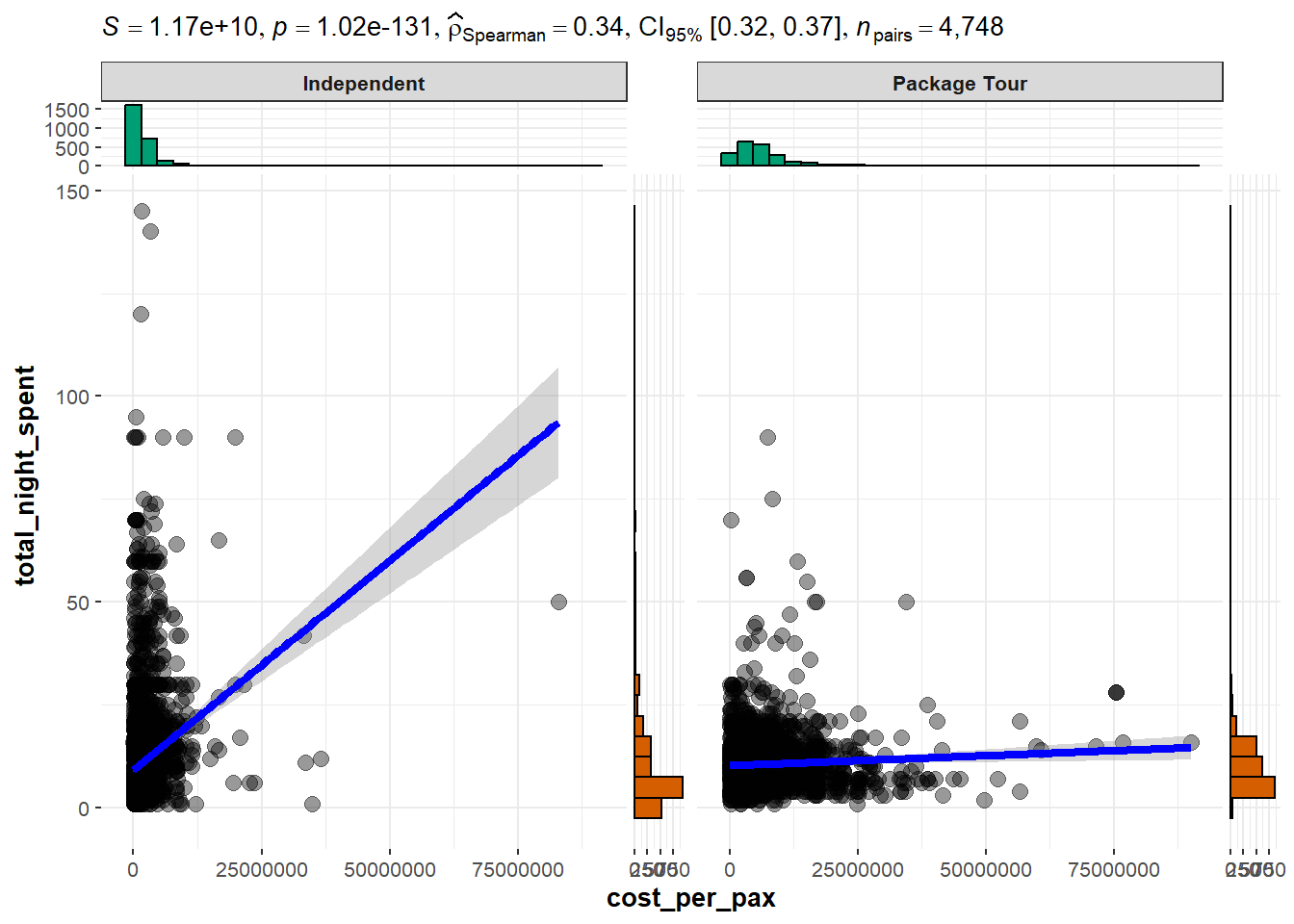

plotcorrelation_costppvtn ("age_group")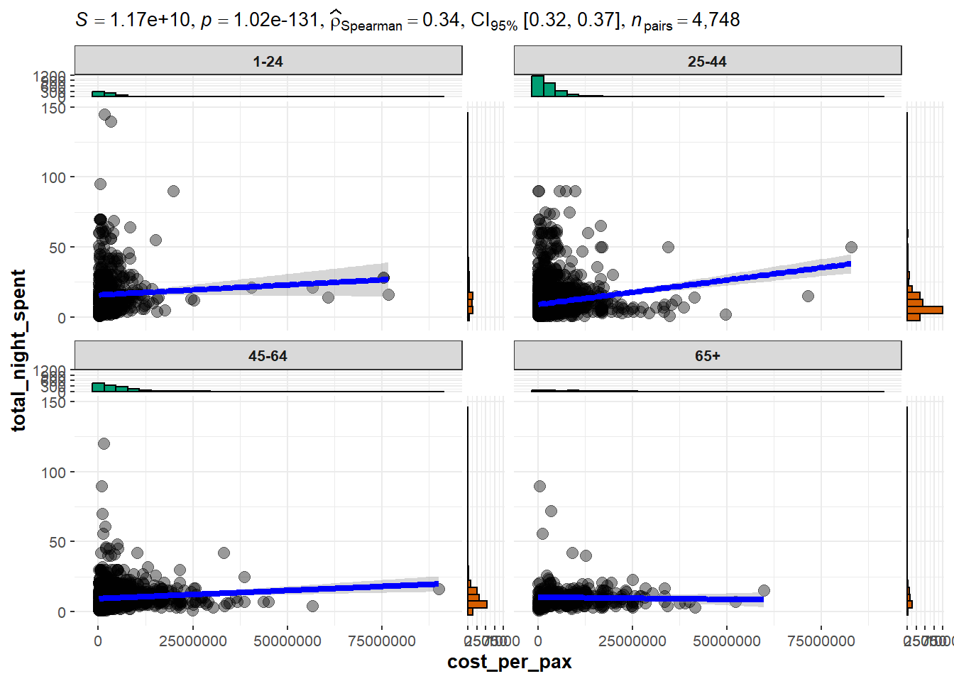

plotcorrelation_costppvtn ("travel_with")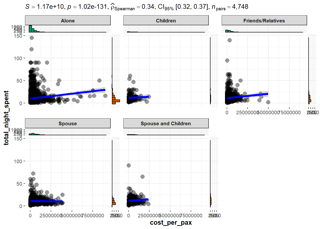

plotcorrelation_costppvtn ("main_activity")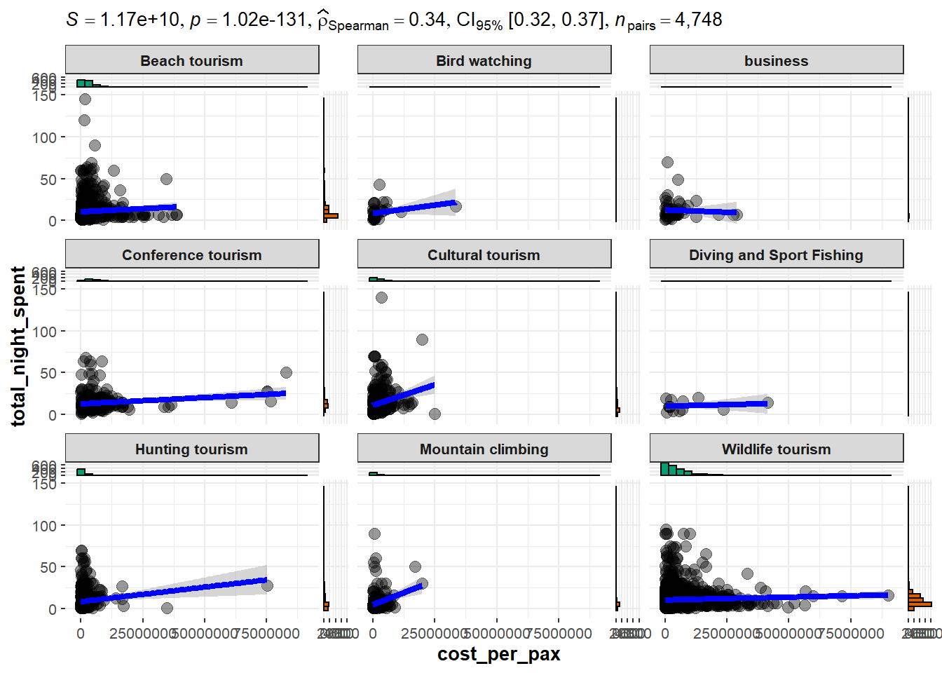

plotcorrelation_costppvtn ("purpose")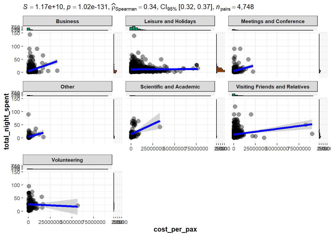

plotcorrelation_costppvtn ("info_source")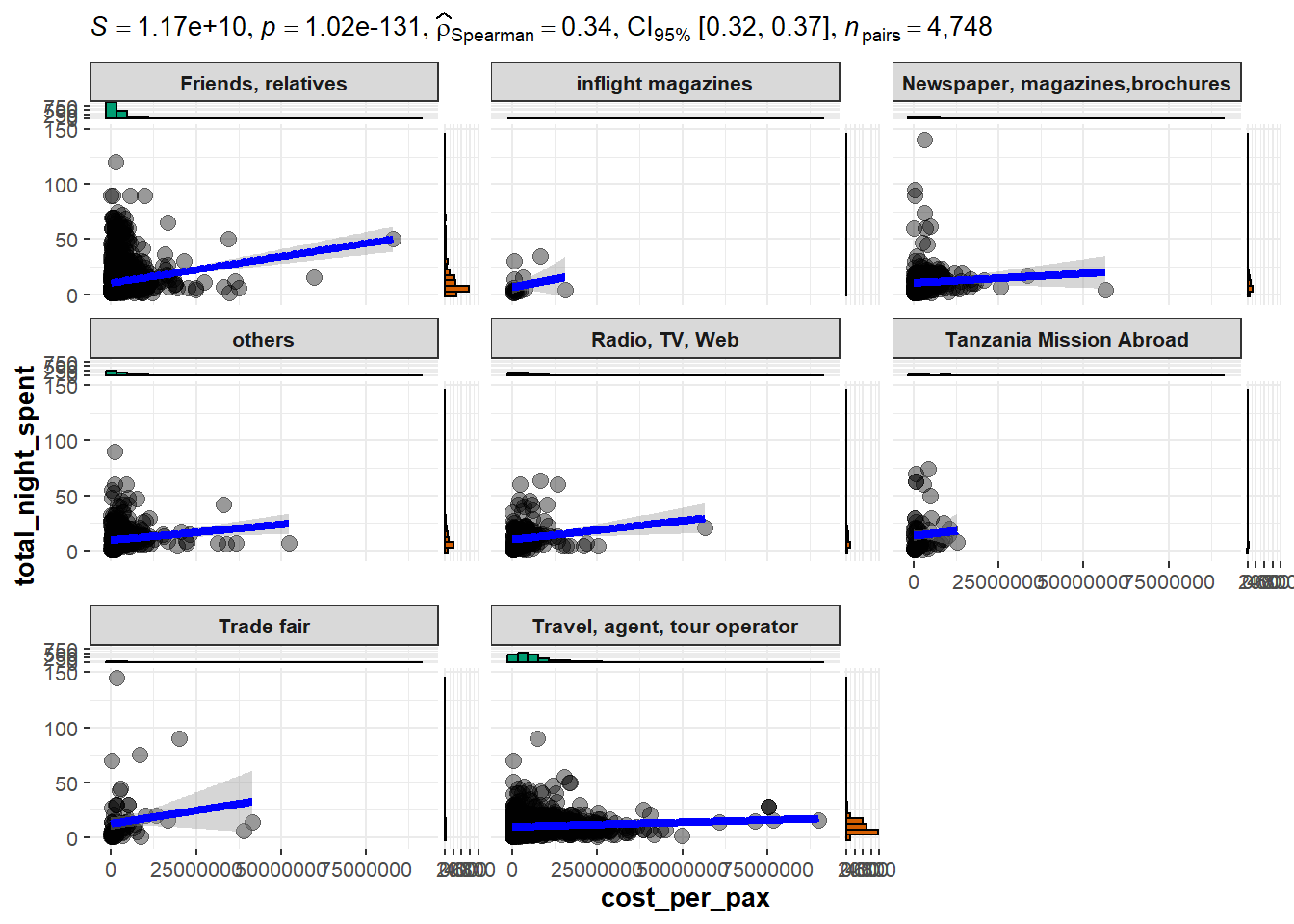

4. Country comparision

options(scipen = 999)

p1 <- ggplot(data = touristdata_clean %>% filter(country == "GERMANY") %>% group_by(tour_arrangement),
                 aes(y = total_cost, x = age_group)) + 
  geom_boxplot(aes(fill = tour_arrangement)) + 
  scale_fill_brewer(palette="YlGnBu") + 
  theme(axis.text.x = element_text(angle = 45, vjust = 1, hjust=1)) + 
  scale_y_continuous(labels = comma)

p1 %>%
  ggplotly() %>%
  layout(boxmode = "group")