pacman::p_load("tmap", "ExPanDaR", "kableExtra", "ggstatsplot", "plotly", "DT", "scales","tidyverse")Confirmatory Data Analysis
1. Installing and launching the required R packages
2. Loading the data
touristdata_clean <- read_csv("data/touristdata_clean.csv")2.1 Adding cost per pax
touristdata_clean <- touristdata_clean %>%
  filter(total_cost > 0,
         total_tourist > 0,
         total_night_spent > 0) %>%
  mutate(cost_per_pax = round(total_cost/total_tourist,0),
         cost_per_night = round(total_cost/total_night_spent,0),
         cost_per_pax_night = round(total_cost/total_tourist/total_night_spent,0))
3. Data overview
3.1 Desriptive Statistics
descr <- prepare_descriptive_table(touristdata_clean %>%
                                       select(!c(14,15,16,17,18,19,20,26))
                                   )


datatable(descr$df, class= "hover") %>%
  formatRound(column = c("Mean", "Std. dev.", "Median"), digits=2)
3.2 Distribution of numerical variables
plot <- touristdata_clean %>%
  select(c(7,8,9,21,22,23,24,28,29,30,31)) %>%
  gather() %>%
  ggplot(aes(value)) +
  facet_wrap( ~key, ncol=4, scales="free") +
  geom_histogram()

ggplotly(plot)
Note:
- Majority spent on mainland
- Mostly travel <5 people
- Spent 5 days on median
3.3 Distribution of categorical variables
plot <- touristdata_clean %>%
  select(c(3,5,6,10,11,12,13,14,15,16,17,18,19,20,25,26,27)) %>%
  gather() %>%
  ggplot(aes(value)) +
  facet_wrap( ~key, ncol=3, scales="free") +
  geom_bar()

ggplotly(plot)
Note:
- Many younger tourist (25-44)
- Info mainly comes from friends and travel agents
- Many comes for wildlife tourism and beach tourism
- Many European and African Tourists
- Many travel alone
- Many comes for leisure and holidays
4. Exploring by Regions and Countries
4.1 Plotting the choropleth map for aggregated metrics
The object World is a spatial object of class sf from the sf package; it is a data.frame with a special column that contains a geometry for each row, in this case polygons
Reference - https://cran.r-project.org/web/packages/tmap/vignettes/tmap-getstarted.html
data("World")touristdata_clean_country <- touristdata_clean %>%
group_by(country,code,region) %>%
summarise(total_female = sum(total_female),
total_male = sum(total_male),
total_tourist = sum(total_tourist),
total_cost = round(sum(total_cost),0),
total_night_spent = round(sum(total_night_spent),0),
cost_per_pax = round(mean(cost_per_pax),0),
cost_per_night = round(mean(cost_per_night),0),
cost_per_pax_night = round(mean(cost_per_pax_night),0),
trips = n()) %>%
mutate(avg_night_spent = round(total_night_spent/trips,0)) %>%
ungroup()Joining the two dataframes together
touristdata_clean_map <- left_join(World,
                                 touristdata_clean_country,
                          by = c("iso_a3" = "code")) %>%
  select(-c(2:15)) %>%
  na.omit()
plot_map_eda <- function(metric = "total_tourist", style = "jenks", classes = 5, minvisitors = 30){
metric_text = case_when(metric == "total_female" ~ "Number of Female Visitors",
metric == "total_male" ~ "Number of Male Visitors",
metric == "total_tourist" ~ "Number of Visitors",
metric == "total_cost" ~ "Total Spending (TZS)",
metric == "cost_per_pax" ~ "Average Individual Spending (TZS)",
metric == "cost_per_night" ~ "Average Spending per Night (TZS)",
metric == "cost_per_pax_night" ~ "Average Individual Spending per Night (TZS)")
tmap_mode("view")
tm_shape(touristdata_clean_map %>%
filter(total_tourist >= minvisitors))+
tm_fill(metric,
n = classes,
style = style,
palette="YlGn",
id = "country",
title = metric_text
) +
tm_borders(col = "grey20",
alpha = 0.5)
}plot_map_eda(metric = "cost_per_pax_night", style = "jenks", classes = 6, minvisitors = 20)Note:
- Majority of tourists come from US, Western Europe, and South Africa
- Many outliers in individual average spending, so only focus on countries with at least 20 visitors, then it’s revealed that Australians spend the highest, followed by Americans and Canadians.
4.2 CDA by Regions
4.2.1 For Numerical Variables
plot_ANOVA_region <- function(metric = "cost_per_pax_night", minvisitors = 30, testtype = "np", pair = "ns", compare = T, conf = 0.95, nooutliers = T) {

metric_text = case_when(metric == "total_female" ~ "Number of Female Visitors",
                        metric == "total_male" ~ "Number of Male Visitors",
                        metric == "total_tourist" ~ "Number of Visitors",
                        metric == "total_cost" ~ "Total Spending (TZS)",
                        metric == "cost_per_pax" ~ "Individual Spending (TZS)",
                        metric == "cost_per_night" ~ "Spending per Night (TZS)",
                        metric == "cost_per_pax_night" ~ "Individual Spending per Night (TZS)",
                        metric == "prop_night_spent_mainland" ~ "Proportion of Night spent in Mainland Tanzania",
                        TRUE ~ metric)

paratext <- case_when(testtype == "p" ~ "Mean (Parametric)",
                      testtype == "np" ~ "Median (Non-Parametric)",
                      testtype == "r" ~ "Mean (Robust t-test)",
                      testtype == "bayes" ~ "Mean (Bayesian)",
                      )

touristdata_countrylist <- touristdata_clean_country %>%
  filter(total_tourist >= minvisitors)

countrylist <- unique(touristdata_countrylist$country)

touristdata_ANOVA <- touristdata_clean %>%
  filter(country %in% countrylist) %>%
  mutate(region = fct_reorder(region, !!sym(metric), median, .desc = TRUE)) %>%
  drop_na()

if(nooutliers == T){
  touristdata_ANOVA <- touristdata_ANOVA %>%
      treat_outliers()
}

touristdata_ANOVA %>%
  ggbetweenstats(x = region, y = !!sym(metric),
                 xlab = "Region", ylab = metric_text,
                 type = testtype, pairwise.comparisons = T, pairwise.display = pair,
                 mean.ci = T, p.adjust.method = "fdr",  conf.level = conf,
                 title = paste0("Comparison of ",paratext," ",metric_text, " across Regions"),
                 package = "ggthemes", palette = "Tableau_10")

}plot_ANOVA_region(metric = "cost_per_pax_night", minvisitors = 30, testtype = "np", pair = "ns", compare = T, conf = 0.95, nooutliers = T)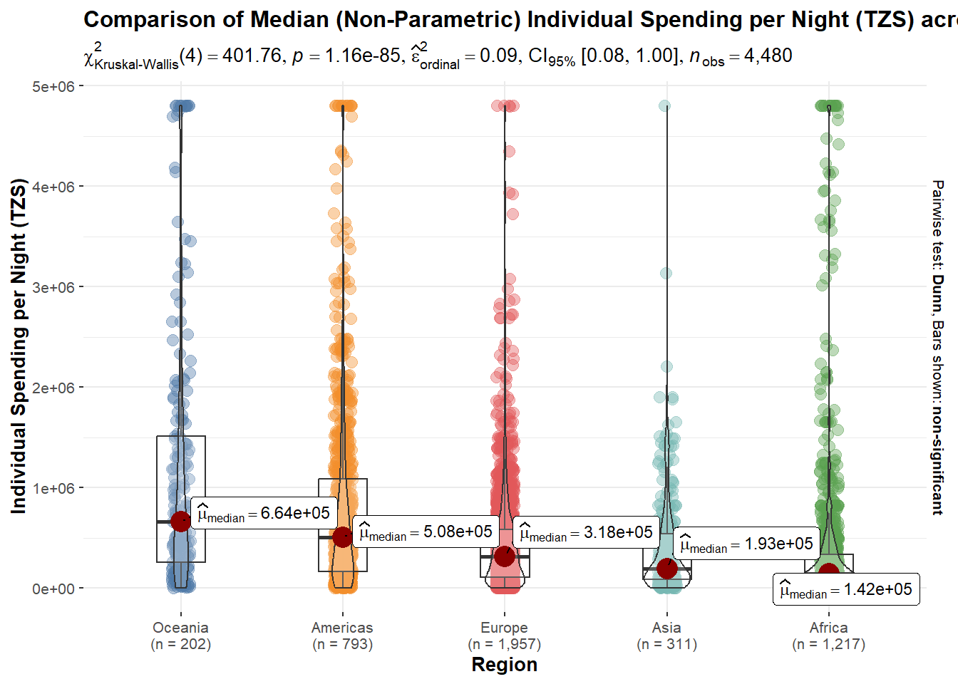
Note: Outliers can be treated Ability to exclude countries with less than minvisitors limit
- Oceania visitors spend the most while African visitors tends to spend the least
plot_ANOVA_region(metric = "prop_night_spent_mainland", minvisitors = 30, testtype = "np", pair = "ns", conf = 0.95)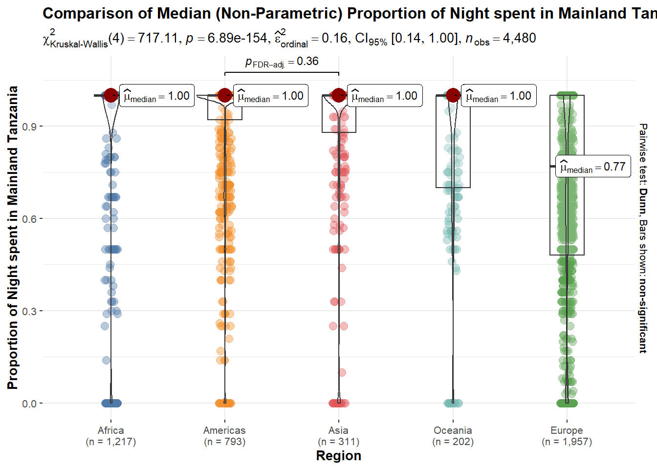
Note : European customers spend more time in Zanzibar
4.2.2 For Categorical Variables
plot_barstats_region <- function(metric = "purpose", minvisitors = 30, testtype = "np",conf = 0.95) {

metric_text = case_when(metric == "age_group" ~ "Age Group",
                        metric == "travel_with" ~ "Travelling Companion",
                        metric == "purpose" ~ "Purpose",
                        metric == "main_activity" ~ "Main Activity",
                        metric == "info_source" ~ "Source of Information",
                        metric == "tour_arrangement" ~ "Tour Arrangement",
                        metric == "package_transport_int" ~ "Include International Transportation?",
                        metric == "package_accomodation" ~ "Include accomodation service?",
                        metric == "package_food" ~ "Include food service?",
                        metric == "package_transport_tz" ~ "Include domestic transport service?",
                        metric == "package_sightseeing" ~ "Include sightseeing service?",
                        metric == "package_guided_tour" ~ "Include guided tour?",
                        metric == "package_insurance" ~ "Insurance Included?",
                        metric == "payment_mode" ~ "Mode of Payment",
                        metric == "first_trip_tz" ~ "First trip to Tanzania?",
                        metric == "most_impressing" ~ "Most impressive about Tanzania?",
                        TRUE ~ metric)

touristdata_countrylist <- touristdata_clean_country %>%
  filter(total_tourist >= minvisitors)

countrylist <- unique(touristdata_countrylist$country)

touristdata_barstats <- touristdata_clean %>%
  filter(country %in% countrylist) %>%
  drop_na()

touristdata_barstats %>%
  ggbarstats(x = !!sym(metric), y = region,
             xlab = "Region", legend.title = metric_text,
             type = testtype, conf.level = conf,
             palette = "Set2")

}plot_barstats_region(metric = "travel_with", minvisitors = 30, testtype = "np", conf = 0.95)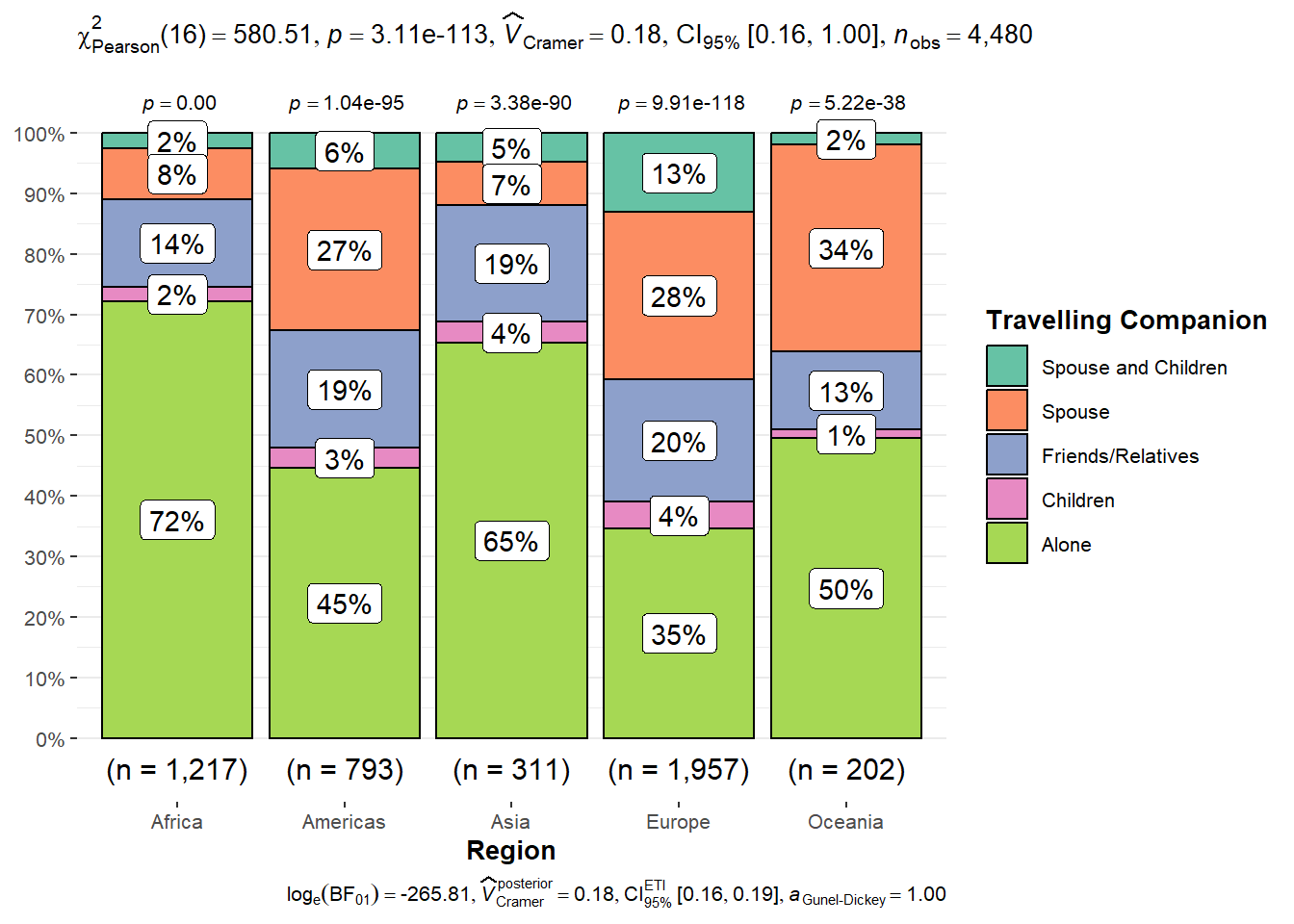
plot_barstats_region(metric = "purpose", minvisitors = 30, testtype = "np", conf = 0.95)
plot_barstats_region(metric = "package_insurance", minvisitors = 30, testtype = "np", conf = 0.95)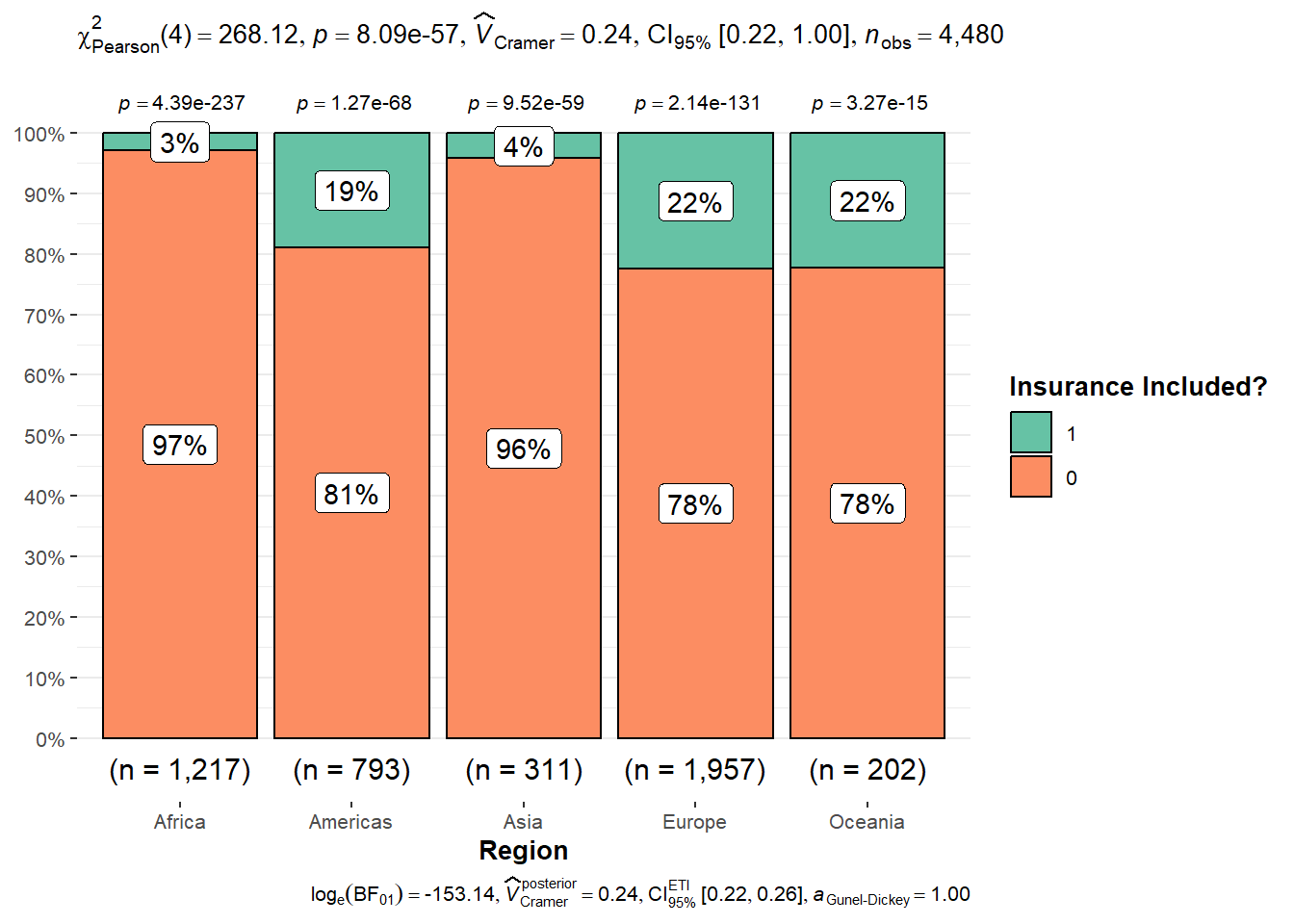
plot_barstats_region(metric = "first_trip_tz", minvisitors = 30, testtype = "np", conf = 0.95)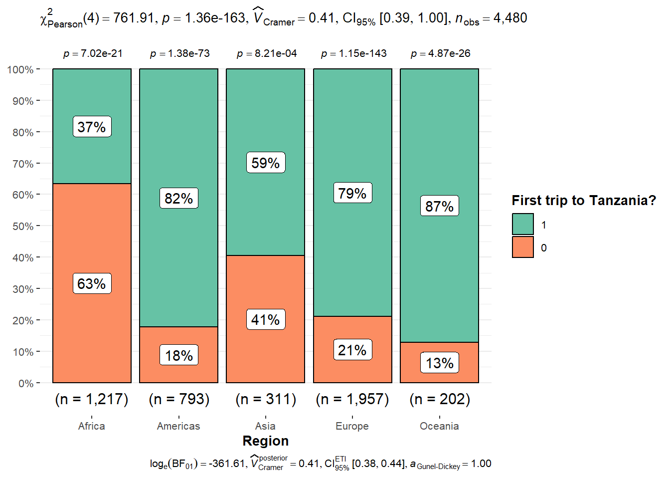
4.3 CDA by Selected Countries
Examining the largest spender by country
touristdata_clean_country_sorted <- touristdata_clean_country %>%
  filter(total_cost > 0,
         total_tourist >= 60) %>%
  arrange(desc(cost_per_pax_night))

top8 <- touristdata_clean_country_sorted$country[1:8]

touristdata_clean_country_sorted
# A tibble: 24 × 13
country code region total…¹ total…² total…³ total…⁴ total…⁵ cost_…⁶ cost_…⁷
<chr> <chr> <chr> <dbl> <dbl> <dbl> <dbl> <dbl> <dbl> <dbl>
1 AUSTRAL… AUS Ocean… 185 126 311 2.72e9 1970 9.58e6 2134147
2 SOUTH A… ZAF Africa 177 258 435 2.57e9 1707 5.78e6 2138016
3 UNITED … USA Ameri… 696 632 1328 8.74e9 7602 7.08e6 1571607
4 CANADA CAN Ameri… 119 88 207 1.42e9 1746 7.45e6 1240173
5 DENMARK DNK Europe 40 34 74 5.97e8 839 1.09e7 914157
6 SWITZER… CHE Europe 74 63 137 7.08e8 849 5.39e6 956006
7 SWEDEN SWE Europe 35 32 67 2.96e8 401 4.93e6 802780
8 SPAIN ESP Europe 230 178 408 1.61e9 1816 4.21e6 1235937
9 ITALY ITA Europe 467 464 931 3.64e9 3888 4.06e6 1049569
10 FRANCE FRA Europe 374 355 729 3.32e9 3581 4.74e6 1169800
# … with 14 more rows, 3 more variables: cost_per_pax_night <dbl>, trips <int>,
# avg_night_spent <dbl>, and abbreviated variable names ¹total_female,
# ²total_male, ³total_tourist, ⁴total_cost, ⁵total_night_spent,
# ⁶cost_per_pax, ⁷cost_per_night4.3.1 For Numerical Variables
plot_ANOVA_country <- function(metric = "cost_per_pax_night", selected_countries, testtype = "np", pair = "ns", compare = T, conf = 0.95, nooutliers = T) {

metric_text = case_when(metric == "total_female" ~ "Number of Female Visitors",
                        metric == "total_male" ~ "Number of Male Visitors",
                        metric == "total_tourist" ~ "Number of Visitors",
                        metric == "total_cost" ~ "Total Spending (TZS)",
                        metric == "cost_per_pax" ~ "Individual Spending (TZS)",
                        metric == "cost_per_night" ~ "Spending per Night (TZS)",
                        metric == "cost_per_pax_night" ~ "Individual Spending per Night (TZS)",
                        metric == "prop_night_spent_mainland" ~ "Proportion of Night spent in Mainland Tanzania",
                        TRUE ~ metric)

paratext <- case_when(testtype == "p" ~ "Mean (Parametric)",
                      testtype == "np" ~ "Median (Non-Parametric)",
                      testtype == "r" ~ "Mean (Robust t-test)",
                      testtype == "bayes" ~ "Mean (Bayesian)",
                      )

touristdata_ANOVA <- touristdata_clean %>%
  filter(country %in% selected_countries) %>%
  mutate(country = fct_reorder(country, !!sym(metric), median, .desc = TRUE)) %>%
  drop_na()

if(nooutliers == T){
  touristdata_ANOVA <- touristdata_ANOVA %>%
      treat_outliers()
}

touristdata_ANOVA %>%
  ggbetweenstats(x = country, y = !!sym(metric),
                 xlab = "Country", ylab = metric_text,
                 type = testtype, pairwise.comparisons = compare, pairwise.display = pair,
                 mean.ci = T, p.adjust.method = "fdr",  conf.level = conf,
                 title = paste0("Comparison of ",paratext," ",metric_text, " across Countries"),
                 package = "ggthemes", palette = "Tableau_10")

}plot_ANOVA_country(metric = "cost_per_pax_night", selected_countries = top8, testtype = "np", pair = "ns", compare = F, conf = 0.95, nooutliers = T)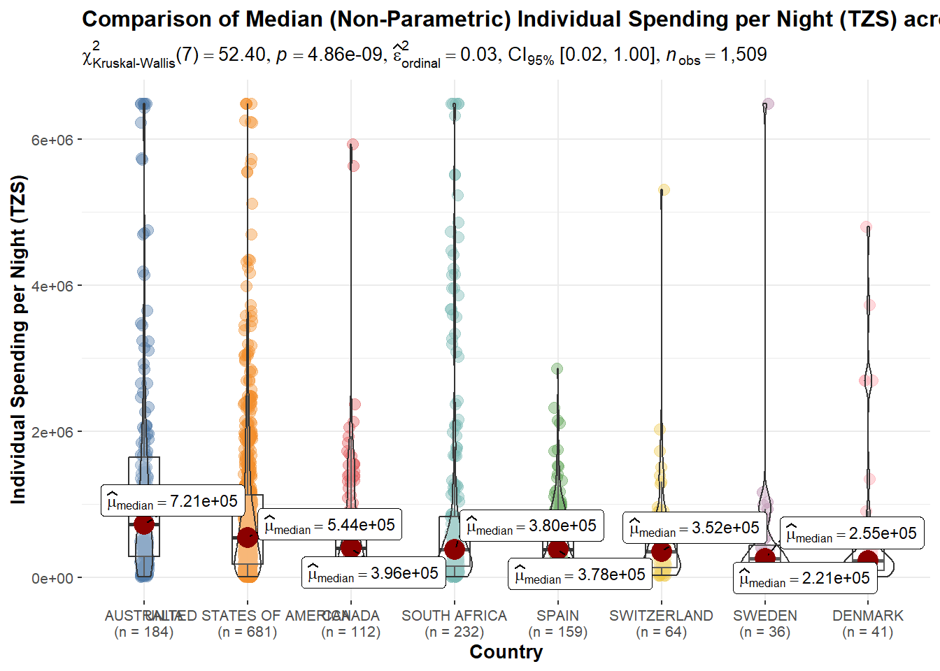
Majority of big spender indeed comes from Australia, followed by US, Canada, New Zealand, Denmark, and South Africa. However, it is noted that there is no statistically significant difference among many of them
plot_ANOVA_country(metric = "prop_night_spent_mainland", selected_countries = top8, testtype = "np", pair = "ns", conf = 0.95)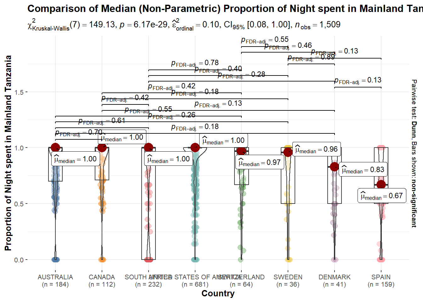
4.3.2 For Categorical Variables
plot_barstats_country <- function(metric = "purpose", selected_countries, testtype = "np",conf = 0.95) {

metric_text = case_when(metric == "age_group" ~ "Age Group",
                        metric == "travel_with" ~ "Travelling Companion",
                        metric == "purpose" ~ "Purpose",
                        metric == "main_activity" ~ "Main Activity",
                        metric == "info_source" ~ "Source of Information",
                        metric == "tour_arrangement" ~ "Tour Arrangement",
                        metric == "package_transport_int" ~ "Include International Transportation?",
                        metric == "package_accomodation" ~ "Include accomodation service?",
                        metric == "package_food" ~ "Include food service?",
                        metric == "package_transport_tz" ~ "Include domestic transport service?",
                        metric == "package_sightseeing" ~ "Include sightseeing service?",
                        metric == "package_guided_tour" ~ "Include guided tour?",
                        metric == "package_insurance" ~ "Insurance Included?",
                        metric == "payment_mode" ~ "Mode of Payment",
                        metric == "first_trip_tz" ~ "First trip to Tanzania?",
                        metric == "most_impressing" ~ "Most impressive about Tanzania?",
                        TRUE ~ metric)


touristdata_barstats <- touristdata_clean %>%
  filter(country %in% selected_countries) %>%
  drop_na()

touristdata_barstats %>%
  ggbarstats(x = !!sym(metric), y = country,
             xlab = "Country", legend.title = metric_text,
             type = testtype, conf.level = conf,
             palette = "Set2")

}plot_barstats_country(metric = "travel_with", selected_countries = top8, testtype = "np", conf = 0.95)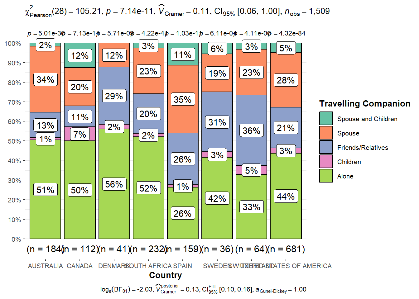
plot_barstats_country(metric = "purpose", selected_countries = top8, testtype = "np", conf = 0.95)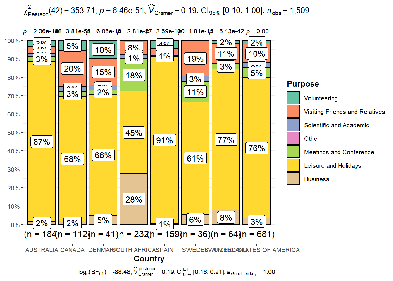
plot_barstats_country(metric = "package_insurance", selected_countries = top8, testtype = "np", conf = 0.95)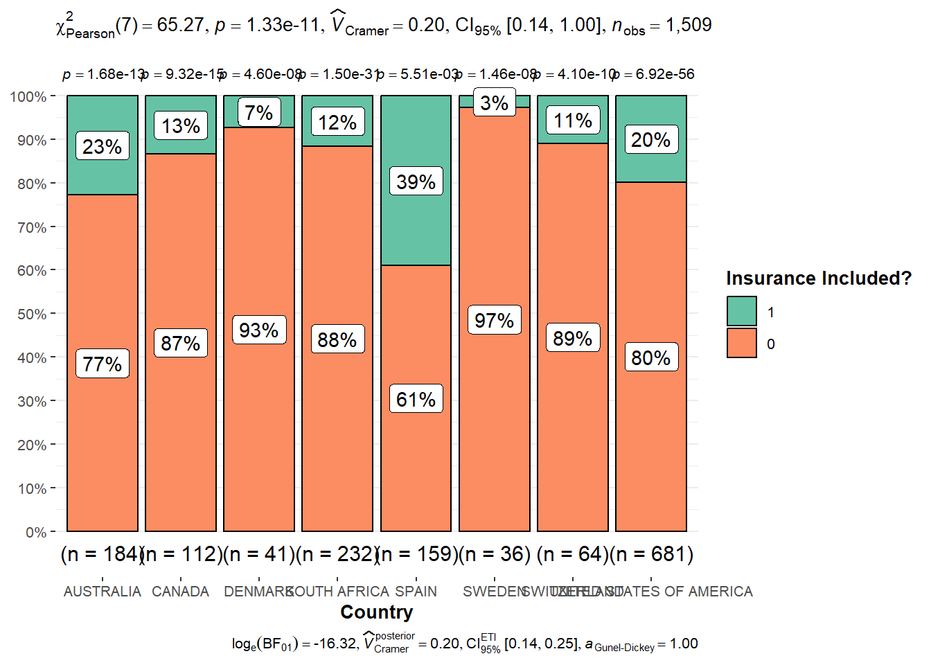
plot_barstats_country(metric = "first_trip_tz", selected_countries = top8, testtype = "np", conf = 0.95)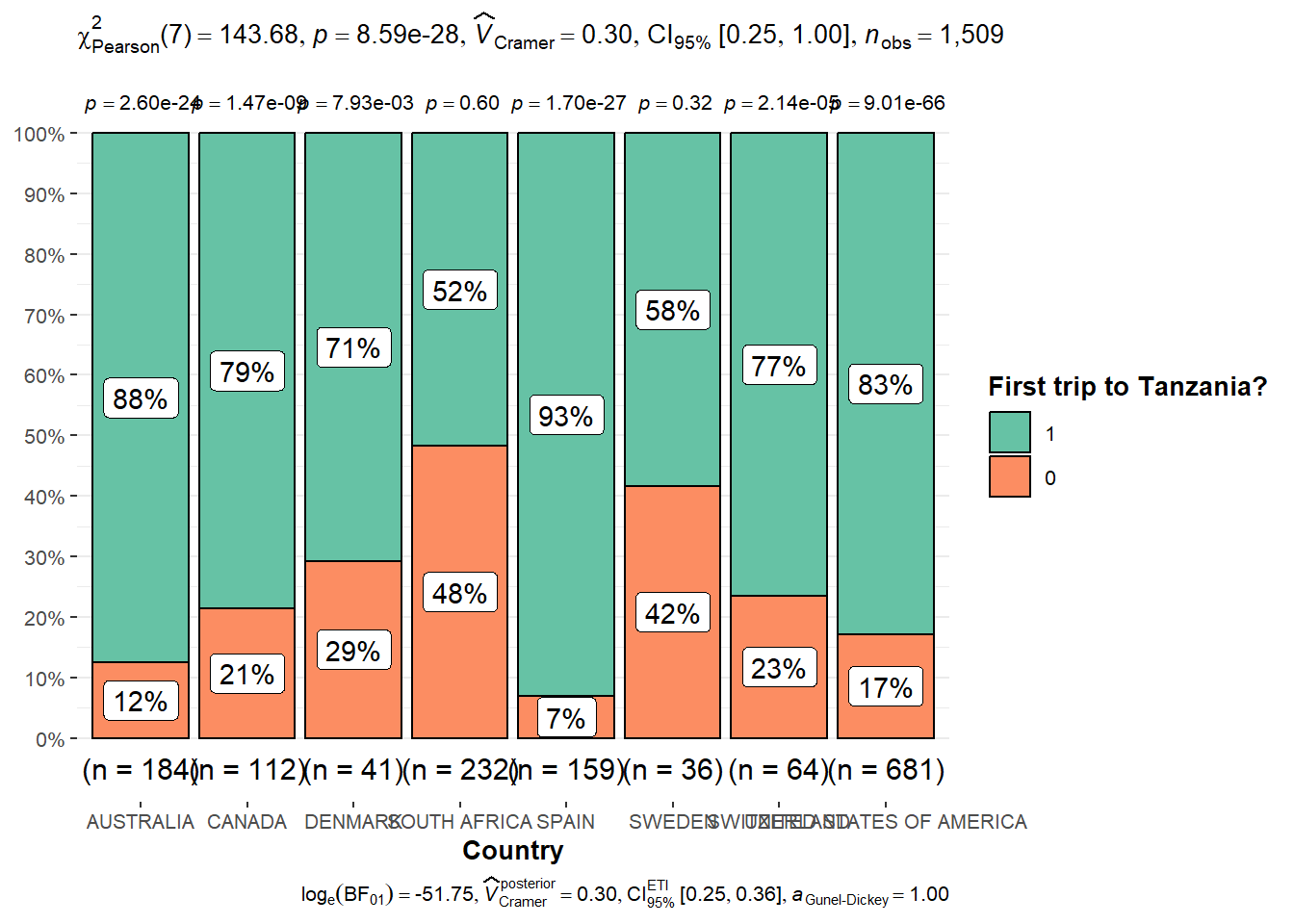
5. Exploring Spending vs Other Variables
5.1 For Numerical Variables
plot_scatter <- function(xaxis = "prop_night_spent_mainland", yaxis = "cost_per_pax_night", regionlist = c("Asia", "Africa", "Europe", "Oceania", "Americas"), max_xaxis, testtype = "np", conf = 0.95, nooutliers = T) {

xaxis_text = case_when(xaxis == "total_female" ~ "Number of Female Visitors",
                       xaxis == "total_male" ~ "Number of Male Visitors",
                       xaxis == "total_tourist" ~ "Number of Visitors",
                       xaxis == "prop_night_spent_mainland" ~ "Proportion of Night spent in Mainland Tanzania",
                       xaxis == "total_night_spent" ~ "Total Night Spent",
                       TRUE ~ xaxis)

yaxis_text = case_when(yaxis == "total_cost" ~ "Total Spending (TZS)",
                       yaxis == "cost_per_pax" ~ "Individual Spending (TZS)",
                       yaxis == "cost_per_night" ~ "Spending per Night (TZS)",
                       yaxis == "cost_per_pax_night" ~ "Individual Spending per Night (TZS)",
                       TRUE ~ yaxis)

if(nooutliers == T){
  touristdata_clean <- touristdata_clean %>%
      treat_outliers()
}

touristdata_clean %>%
  filter(region %in% regionlist,
         !!sym(xaxis) <= max_xaxis) %>%
  ggscatterstats(x = !!sym(xaxis), y = !!sym(yaxis),
                 type = testtype, conf.level = conf) +
  theme(axis.text.x = element_text(angle = 45, vjust = 1, hjust=1)) +
  labs(x = xaxis_text, y = yaxis_text)

}plot_scatter(xaxis = "total_tourist", yaxis = "total_cost", regionlist = c("Europe","Americas","Oceania"), max_xaxis = 100, testtype = "np", conf = 0.95, nooutliers = T)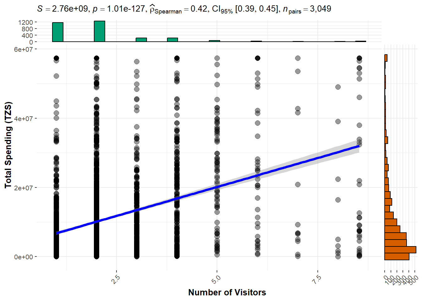
5.2 For Categorical Variables
plot_ANOVA <- function(xaxis = "age_group", yaxis = "total_cost", regionlist = c("Asia", "Africa", "Europe", "Oceania", "Americas"), testtype = "np", pair = "ns",conf = 0.95, nooutliers = T) {

xaxis_text = case_when(xaxis == "age_group" ~ "Age Group",
                        xaxis == "travel_with" ~ "Travelling Companion",
                        xaxis == "purpose" ~ "Purpose",
                        xaxis == "main_activity" ~ "Main Activity",
                        xaxis == "info_source" ~ "Source of Information",
                        xaxis == "tour_arrangement" ~ "Tour Arrangement",
                        xaxis == "package_transport_int" ~ "Include International Transportation?",
                        xaxis == "package_accomodation" ~ "Include accomodation service?",
                        xaxis == "package_food" ~ "Include food service?",
                        xaxis == "package_transport_tz" ~ "Include domestic transport service?",
                        xaxis == "package_sightseeing" ~ "Include sightseeing service?",
                        xaxis == "package_guided_tour" ~ "Include guided tour?",
                        xaxis == "package_insurance" ~ "Insurance Included?",
                        xaxis == "payment_mode" ~ "Mode of Payment",
                        xaxis == "first_trip_tz" ~ "First trip to Tanzania?",
                        xaxis == "most_impressing" ~ "Most impressive about Tanzania?",
                        TRUE ~ xaxis)

yaxis_text = case_when(yaxis == "total_cost" ~ "Total Spending (TZS)",
                       yaxis == "cost_per_pax" ~ "Individual Spending (TZS)",
                       yaxis == "cost_per_night" ~ "Spending per Night (TZS)",
                       yaxis == "cost_per_pax_night" ~ "Individual Spending per Night (TZS)",
                       TRUE ~ yaxis)


touristdata_ANOVA <- touristdata_clean %>%
  filter(region %in% regionlist) %>%
  drop_na()

if(nooutliers == T){
  touristdata_ANOVA <- touristdata_ANOVA %>%
      treat_outliers()
}

touristdata_ANOVA %>%
  ggbetweenstats(x = !!sym(xaxis), y = !!sym(yaxis),
                 xlab = xaxis_text, ylab = yaxis_text,
                 type = testtype, pairwise.comparisons = T, pairwise.display = pair,
                 mean.ci = T, p.adjust.method = "fdr",  conf.level = conf,
                 package = "ggthemes", palette = "Tableau_10")

}plot_ANOVA(xaxis = "travel_with", yaxis = "total_cost", regionlist = c("Asia", "Africa", "Europe", "Oceania", "Americas"), testtype = "np", pair = "ns",conf = 0.95, nooutliers = T)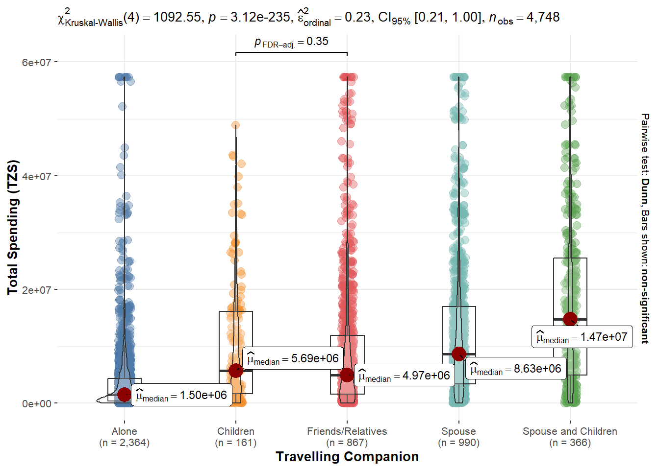
plot_ANOVA(xaxis = "age_group", yaxis = "total_cost", regionlist = c("Asia", "Africa", "Europe", "Oceania", "Americas"), testtype = "np", pair = "ns",conf = 0.95)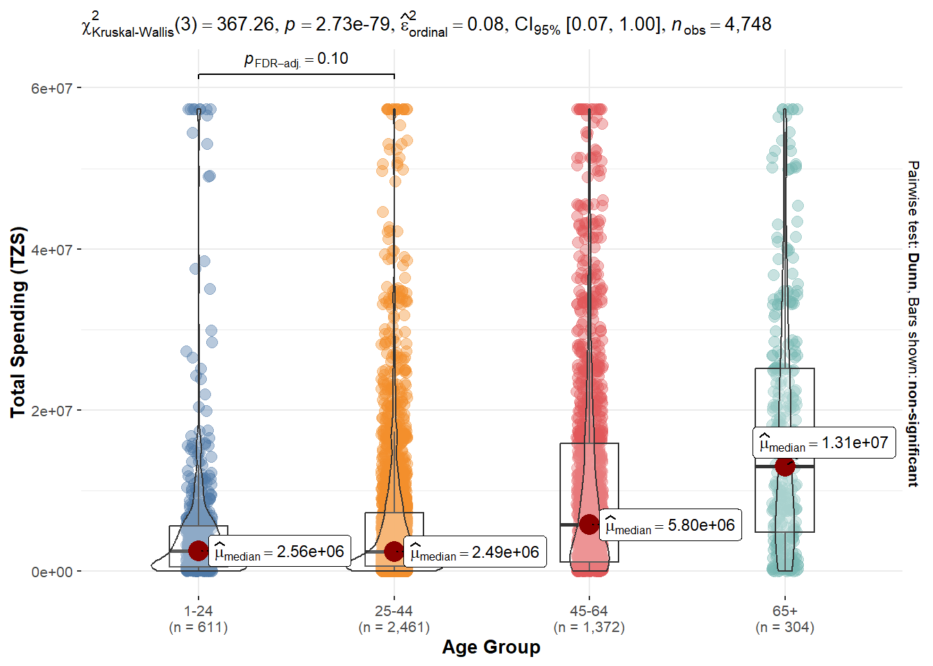
plot_ANOVA(xaxis = "purpose", yaxis = "total_cost", regionlist = c("Asia", "Africa", "Europe", "Oceania", "Americas"), testtype = "np", pair = "ns",conf = 0.95)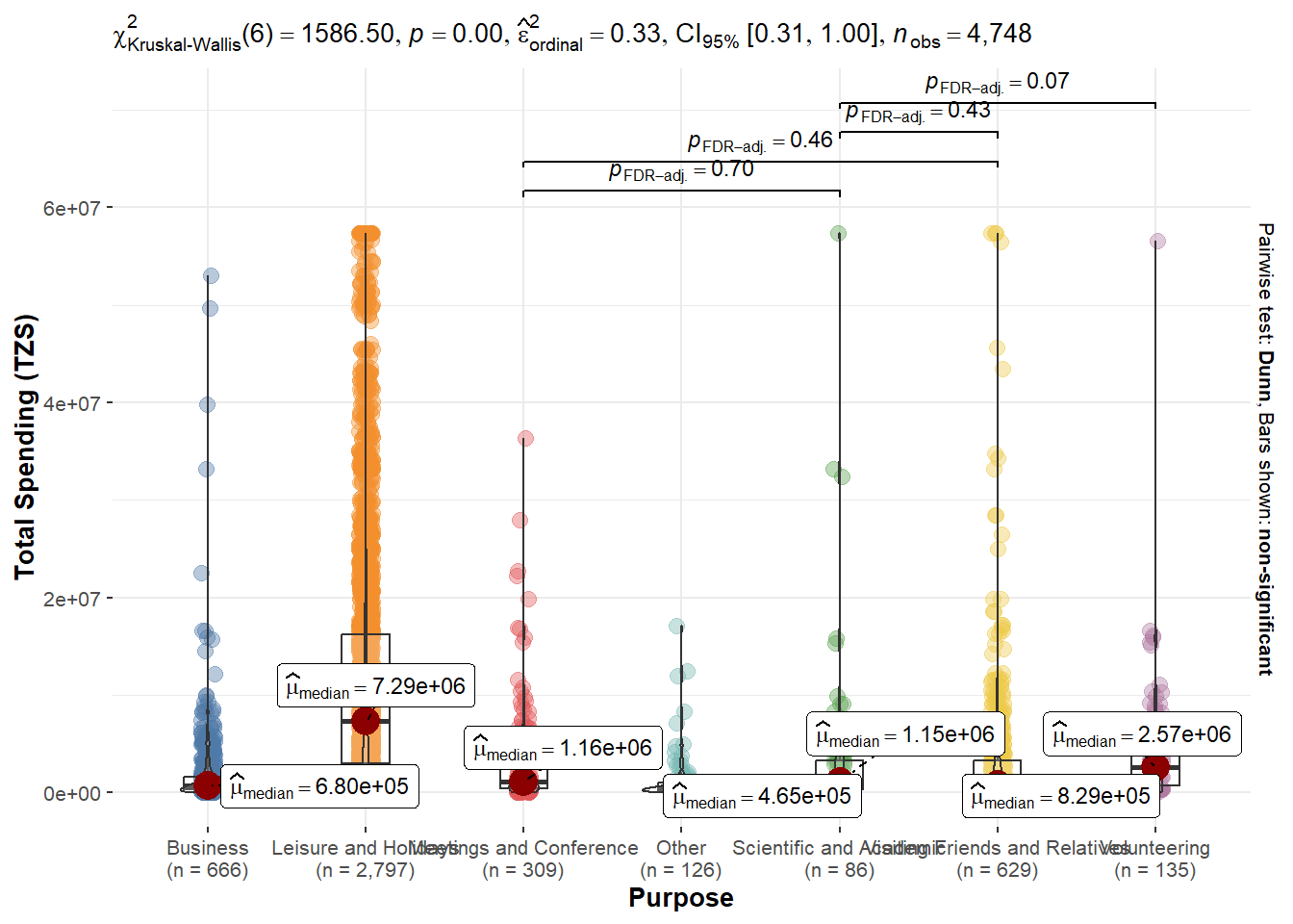
6. Exploring Other Variables
plot_barstats <- function(xaxis = "age_group", yaxis = "purpose", regionlist = c("Asia", "Africa", "Europe", "Oceania", "Americas"), testtype = "np",conf = 0.95) {

xaxis_text = case_when(xaxis == "age_group" ~ "Age Group",
                        xaxis == "travel_with" ~ "Travelling Companion",
                        xaxis == "purpose" ~ "Purpose",
                        xaxis == "main_activity" ~ "Main Activity",
                        xaxis == "info_source" ~ "Source of Information",
                        xaxis == "tour_arrangement" ~ "Tour Arrangement",
                        xaxis == "package_transport_int" ~ "Include International Transportation?",
                        xaxis == "package_accomodation" ~ "Include accomodation service?",
                        xaxis == "package_food" ~ "Include food service?",
                        xaxis == "package_transport_tz" ~ "Include domestic transport service?",
                        xaxis == "package_sightseeing" ~ "Include sightseeing service?",
                        xaxis == "package_guided_tour" ~ "Include guided tour?",
                        xaxis == "package_insurance" ~ "Insurance Included?",
                        xaxis == "payment_mode" ~ "Mode of Payment",
                        xaxis == "first_trip_tz" ~ "First trip to Tanzania?",
                        xaxis == "most_impressing" ~ "Most impressive about Tanzania?",
                        TRUE ~ xaxis)

yaxis_text = case_when(yaxis == "age_group" ~ "Age Group",
                        yaxis == "travel_with" ~ "Travelling Companion",
                        yaxis == "purpose" ~ "Purpose",
                        yaxis == "main_activity" ~ "Main Activity",
                        yaxis == "info_source" ~ "Source of Information",
                        yaxis == "tour_arrangement" ~ "Tour Arrangement",
                        yaxis == "package_transport_int" ~ "Include International Transportation?",
                        yaxis == "package_accomodation" ~ "Include accomodation service?",
                        yaxis == "package_food" ~ "Include food service?",
                        yaxis == "package_transport_tz" ~ "Include domestic transport service?",
                        yaxis == "package_sightseeing" ~ "Include sightseeing service?",
                        yaxis == "package_guided_tour" ~ "Include guided tour?",
                        yaxis == "package_insurance" ~ "Insurance Included?",
                        yaxis == "payment_mode" ~ "Mode of Payment",
                        yaxis == "first_trip_tz" ~ "First trip to Tanzania?",
                        yaxis == "most_impressing" ~ "Most impressive about Tanzania?",
                        TRUE ~ yaxis)


touristdata_barstats <- touristdata_clean %>%
  filter(region %in% regionlist) %>%
  drop_na()

touristdata_barstats %>%
  ggbarstats(x = !!sym(yaxis), y = !!sym(xaxis),
             xlab = xaxis_text, legend.title = yaxis_text,
             type = testtype, conf.level = conf,
             palette = "Set2")

}plot_barstats(xaxis = "age_group", yaxis = "purpose", regionlist = c("Asia", "Africa", "Europe", "Oceania", "Americas"), testtype = "np",conf = 0.95)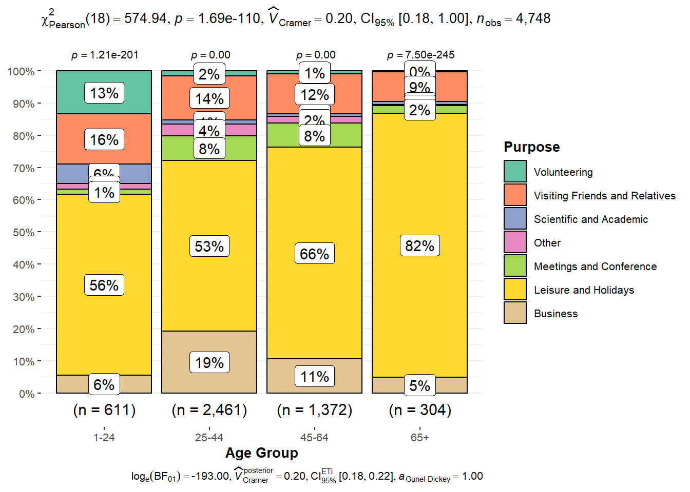
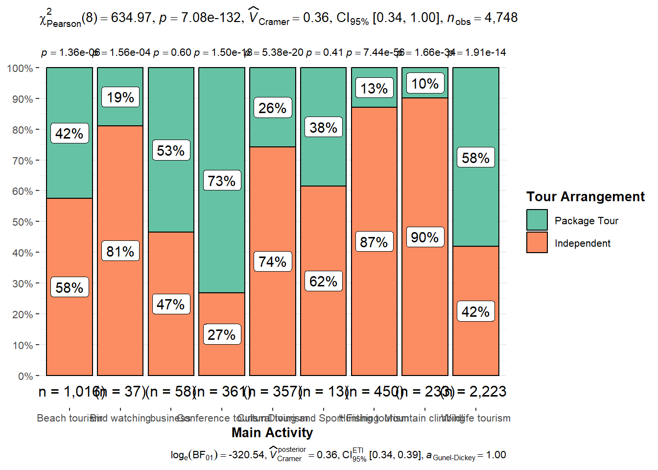
plot_barstats(xaxis = "main_activity", yaxis = "tour_arrangement", regionlist = c("Asia", "Africa", "Europe", "Oceania", "Americas"), testtype = "np",conf = 0.95)